Image compression
By transform coding
The recent section on image compression is enhanced by introducing transform coding for demanding subblocks.
The 'gif' and 'jpeg' standards provide very good results most of the time. However, being inquisitive and trying out different versions has never hurt any project.
Vector quantisation and quadtree decomposition have already been discussed in the recent compression section.
For the purposes of this section, a transform converts spatial (or temporal) data into a frequency spectrum. It does not automatically provide data compaction. However, high frequency components are either represented using a lower number of bits, or omitted altogether, and then there is the potential for data compression.
A transform is usually more effective for a rather larger block size than the 4x4 used in this compression series. This will better amortise the overheads of storing the serial numbers of waves to be retained and, in this program, the coordinates of the top left corner of the demanding subblock.
The point made in relation to dynamic quadtrees (having uneven, rather than equal, partitions) bears repeating: It should be the particular block which decides how many, and which components are retained, not the programmer: It sure needs more work. From some point onwards, though, compression factors, reconstruction quality and algorithm simplicity cannot be improved independently of each other.
Transform compression will not be as good as pattern matching for computer generated images, so this project may seem a bit of 'much ado about nothing'. For more detailed images, though, like photographs, it is a different matter: It may well be that transform coding will lead to fewer demanding partitions being losslessly encoded as a last resort.
The same image is used for all tests. Four settings of the quality control are displayed:
Lossless |
Error: Actual average~ 0.1% |
Error:~ 0.2%. |
Error:~ 0.3%
|
The following table displays compressed file sizes against actual average and maximum acceptable error. The size of the simplified bitmap was 16,386 bytes:
| Size | actual error (%) | max error (%) |
| 5911 | Loss free | 0.2 |
| 5564 | 0.1 | 1 |
| 5444 | 0.2 | 1.5 |
| 5378 | 0.25 | 1.8 |
| 5322 | 0.3 | 2 |
Several different images should be tested before claiming compression figures. The compression factor for the image above is about 3 times for an actual average error of 0.3%.
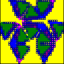
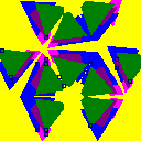
The decimation maps for demanding compartments are shown next: Both transform coded subblocks (top) and losslessly encoded partitions are shown.


A true transform has not been implemented in this section: The twin frequency has been left out, in favour of an additional low sequency component, in line with the ideas listed in the last section. (It is easy to add the former, too, though.)
The average value of the row, plus, if need be, the prevailing component, are only retained. This means that the row of four pixels should basically have two colours, and only one, or zero (rather than 2 or 3) boundaries can be exactly represented. The colour pairs can be different for each of the three adjacent rows. For 4x4 blocks, this is not asking a lot, and if it fails by more than the margin preset, the partition can always be encoded losslessly, anyway.
This can be seen not to provide much compression worth speaking of. However, almost half of the adjacent rows have much the same coefficients. The redundancy is begging to be exploited and the program obliges!
The ‘transform’ subroutine performs most of the transform coding process. The number of bytes in the transform coded block follows the corresponding figure for losslessly encoded partitions (two bytes.) Lastly, the transform coding section is appended to the compression file. It has the format detailed below:
- location of top left corner (2 bytes)
- the position of the row boundary (1-3) or 0 to signify a uniform row. A value of 4 implies coefficients are copied from the row just above. (1 byte)
- the values of the corresponding colours from left to right (0,1, or 2 bytes according to the position of the boundary)
The transform subroutine has been written so as to try a new version fast. It looks at different cases, rather than being easy to modify if someone decided to switch, say, to an 8x8 demanding subblock size. This isn't really acceptable, and I am not proud of this routine. An improved version is promised in the future.
When one side of a boundary involves 3 pixels, a majority rule is tried before the mean value: This hopefully avoids introducing colours which did not exist in the unprocessed picture (for black and white, there is probably no need to bother.) Unfortunately, this also makes the routine longer than I would have liked.
The shortcuts in the original version are still present, regrettably, for now: The input file is in a simplified bitmap format, and only square images are handled- the number of pixels on a side is an integer power of two. The input image is expected to be in 'image.bin' in the default directory used by the language for its files. Compression data is put to the 'compress.bin' file in the same directory, overwriting any existing file of the same name. The source code for this section is supplied.
Initially, compression is easily obtained. The programmer, however, will probably have to struggle for each improvement thereafter.
The site will let the subject of image compression rest, for some time. Still, it hasn't discussed several important issues in detail:
- Packing more pixels in a byte, when the maximum number of colours is 16, 4 or 2
- Adaptive quadtrees (having unequal partitions.) It will make a difference, mainly for computer generated images.
- It is a moot point to faithfully represent random noise on a rough surface. (Admittedly, this is getting into the area of the criteria for accepting the compression of a block which may not seem entirely objective.) The improvements will be seen chiefly in photographs, rather rather than pictures created by computers.
More links:
