My experiments with chaos

My experiments with chaos
If you are interested in chaos, you surely know already about the logistic equation (and if you don't, look here ). The idea is quite simple: a mathematical model to represent a population of, let's say, rabbits. The formula is quite simple, too:

Rnew=R+a*R-b*R^2

where:

Rnew is the new rabbit population (after one year, one month, or any other amount of time you think reasonable)
R is the old rabbit population
a*R is the number of new-born rabbits, proportional to the number of existing rabbits
b*R^2 is the number of rabbits that die. We take R squared because we want to represent that when there are too many rabbits, there won't be enough food for all of them, so there will be many more deaths when R is high.

After I learned that this simple formula could lead to the most surprising results (and again, this is your last chance if you don't know already), I decided to experiment a little. What if there are foxes in the area? We'd need to change the equation and add a new one for the foxes, like this:

Rnew=R+a*R-b*R^2-c*R*F
Fnew=F-d*F+e*R*F

where

Rnew is the new rabbit population
R is the old rabbit population
a*R is the number of new-born rabbits
b*R^2 is the number of rabbits that die from natural causes
c*R*F is the number of rabbits eaten by foxes, that depends both on the number of existing rabbits and the number of existing foxes.
Fnew is the new fox population
F is the old fox population
d*F is the number of foxes that die
e*R*F is the number of new-born foxes. The idea is: the more rabbits are eaten, the more foxes are born.

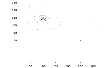
In this phase diagram, each pair of values (rabbits, foxes) is represented with a point. As you can see, here the two populations oscillate until they finally reach an equilibrium point. This is a bit boring, and as the logistic equation is part of the system, I expected that more exciting, chaotic things would happen if I played with the values of the constants a, b, c, d and e.

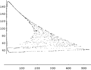
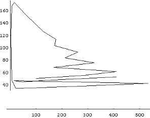
After a few experiments, I found a situation in which the two populations followed a cycle that never repeated exactly. Plotting the points during many seasons, I got this wrinkled curve. This is a sure sign of a strange attractor lying near... I didn't take long to find it; you can see two of them below.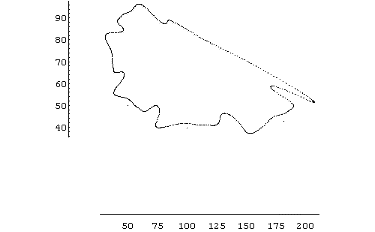

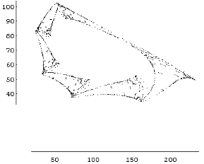
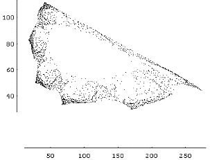
Until now, nothing really unexpected had happened. The equations I had used are already well-known: they are called Lotke-Volterra equations, so probably these attractors have already been found and studied in some University. But from now on, we'll move into unexplored realms.

A friend wondered if the Lotke-Volterra equations were realistic enough. The reproduction of foxes shouldn't be substantially different from the reproduction of rabbits (only, perhaps, at a slower rate). But the death rate of foxes should be influenced by the number of rabbits (foxes will starve if there aren't any rabbits, won't they?). Considering this, I changed the second equation to:

Fnew=F-d*F/R+e*F

where

Fnew is the new fox population
F is the old fox population
d*F/R is the number of foxes that die. The less rabbits, the more foxes will die.
e*F is the number of new-born foxes.

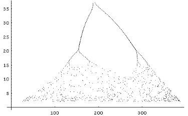This is what I got in my first plot. It looks like a bifurcation diagram, doesn't it? Now, one thing is getting a bifurcation diagram after following carefully the instructions to plot one, and a very different thing is getting a bifurcation diagram from a set of equations that should yield something like a cycle. What on earth is happening here?

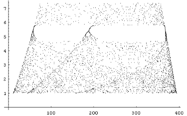
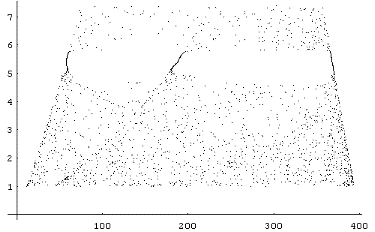
After studying carefully the situation, I realized that the "rabbits" equation is almost the logistic equation, only with one added term, that depends on the number of foxes. I had given "d" a very small value, which means that the number of foxes just kept increasing, regardless of the number of rabbits. Result: the two equations could be reduced to a logistic equation whose parameters changed slowly with time. So it's not so surprising that I got a bifurcation diagram! Setting d=0, to eliminate feedback between F and R, I could get some fast, good pictures. This method of drawing the bifurcation diagram has its advantages: first, it's faster than the usual one, because there's no need to wait for the transients to pass. Second, it allows us to explore the bifurcation diagram in new ways. For example, plotting only one of every second point, one could see the bifurcation diagram lose one of its branches. In the period-three window, each one of the bifurcations also lose one of the branches!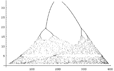

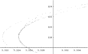But let's not forget what I was after when I modified the equations. Giving the constants more reasonable values, I found what I was looking for: a strange attractor. But this one is rather interesting. As you can see, the right side of the loop always follows the same path, but the left side "goes wild" (in the second figure you can see one of these loops). I have never seen anything like this before, but maybe that's only my ignorance.

And here's the last discovery. I started wondering if that line to the left was what it appeared to be. After all, strange attractors should be fractal, and lines aren't very fractal. So I zoomed and zoomed and - there you are! This is a magnification of that line (it seems very curved because it's much more magnified in the horizontal direction - look at the scale!)

If you are interested in these equations, or just would like to know the exact values of the constants that produced each plot to repeat them at home, you can e-mail me at lusina@redestb.es

Back to the Math page